2024-11-26
Introduction to Big O Notation
Now it’s time to touch this important topic in computer science. But to understand these concepts you’ve to know about Time and Space Complexity and the basics about memory. Once you have that knowledge we’re ready to start
Big O Notation
Is a mathematical notation that describes the limiting behavior of a function when the argument tends towards a particular value or infinity. In computer science, big O notation is used to classify algorithms according to how their run time or space requirements grow as the input size grows.
In simple terms we can use the big O notation to measure how good an algorithm is based on the time that takes to execute (in seconds) and the space (in memory) that needs to execute. It’s not the same if you have an array of 10 elements and you need to iterate over it than if you have the very same array but with 100.000 elements. Both operations will take different amounts of time and space and we have a way to measure it. Pay attention here because we’re talking about iterating through a simple array of numbers, not about other kinds of operations like ordering from ascending to descending order (which actually can take a different amount of time and space)
N
Following the example mentioned above where we have an array of 10 or 100.000 numbers, any of them can be denoted as the “N” character. This means that if you have just 1 element in the arrays, it doesn't matter the operation itself, because it will execute almost instantly. But if we increment the “N” to 100.000 it completely change the time and space that takes to execute
O(1) - Constant Time
First algorithm
2.6.8 :016 > array = [1, 2, 3, 4]
=> [1, 2, 3, 4]
2.6.8 :017 > operation_1 = array[0] * 10
=> 10
This operation is a simple creation of an array of 4 elements and then we select the first position of the array and we multiply it by 10
In our previous example is the first algorithm, which will be always executed in constant time. It doesn't matter the number of the elements of the array. Why is that? Because we’re just selecting the first element of the array and then we multiplied by 10. So it doesn’t matter the number of elements in the array. This is the Holy Grail, but this is the elemental operation, which just happens in the cases similar to the mentioned one.
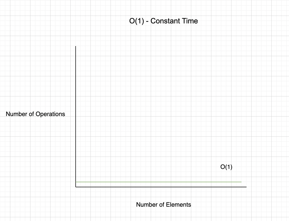 Constant Time
Of course all of this explanation is at a high level, if you want to learn more about constant time please click here.
O(n) - Linear Time
Second algorithm
2.6.8 :018 > operation_2 = array.each {|a| puts a}
1
2
3
4
=> [1, 2, 3, 4]
In this operation we used the same array created before, and iterate through each element of the array and then printed out
In our previous example is the second algorithm, which will be executed in “linear time”. As we mentioned above the “n” is the number of elements of the array (in our example). So if we have 4 elements it will take 0(4) time and space complexity and if we have 100.000 elements it will take 0(100000) time and space. I think you got it, it's a matter of the size of the array and the operation itself: a simple iteration. The most common use cases here are:
* Simple iteration over array.length
* Loop over a simple collection of elements
* Iterate over half a collection of elements
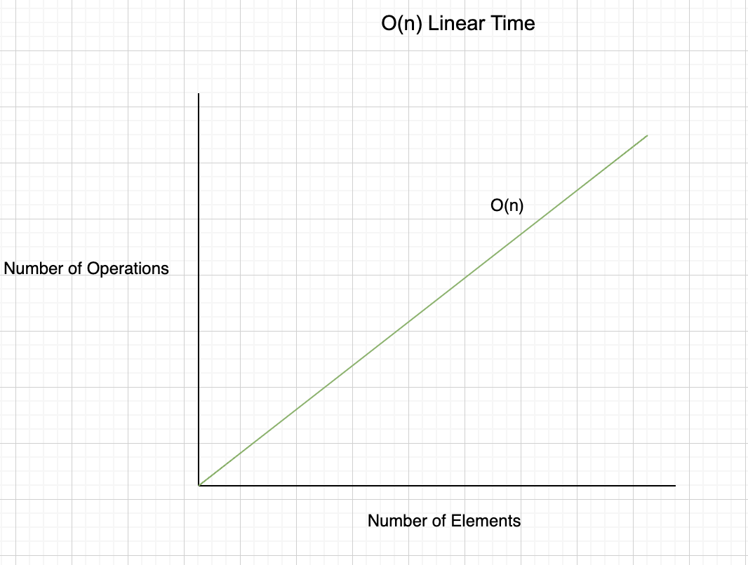 Linear Time
Of course all of this explanation is at a high level, if you want to learn more about constant time please click here.
O(n**2) - Quadratic Time
Third algorithm
2.6.8 :019 > operation_3 = array.each do |a1|
2.6.8 :020 > array.each do |a2|
2.6.8 :021 > puts a1 * a2
2.6.8 :022?> end
2.6.8 :023?> end
1
2
3
4
2
4
6
8
3
6
9
12
4
8
12
16
=> [1, 2, 3, 4]
And the last algorithm goes 2 times through the same array of 4 elements and multiplies each element of each iteration.
As we said before we have now just 4 elements inside the array, but if we increase that number of elements to be 100.000 or even 1 million elements, the time and space that takes to execute will change drastically between the 3
In our previous example is the third algorithm, which will be executed in “quadratic time”. Because we’re iterating two times the very same array we have to square the “n” elements of the array. So if we have 4 elements it will take 0(4**2) time and space complexity and if we have 100.000 elements it will take 0(100000**2) time and space. Here is where the algorithm starts to take much more time and space to be executed. The most common use cases here are:
* The handshake problem
* Two nested for loops iterating over the same collection
* Every element has to be compared to every other element
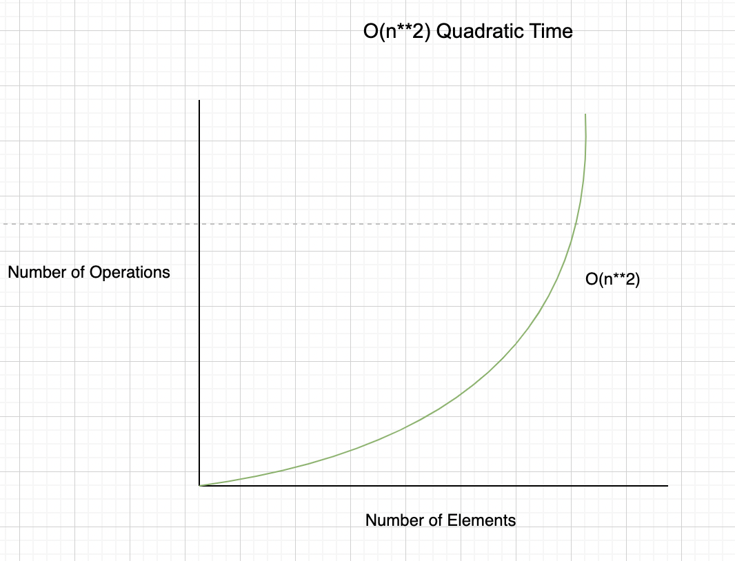 Quadratic Time
Other Notations Cheatsheet
There are certainly many more notations than mentioned before. Take at time to try to understand the other ones and you can find more on next resources:
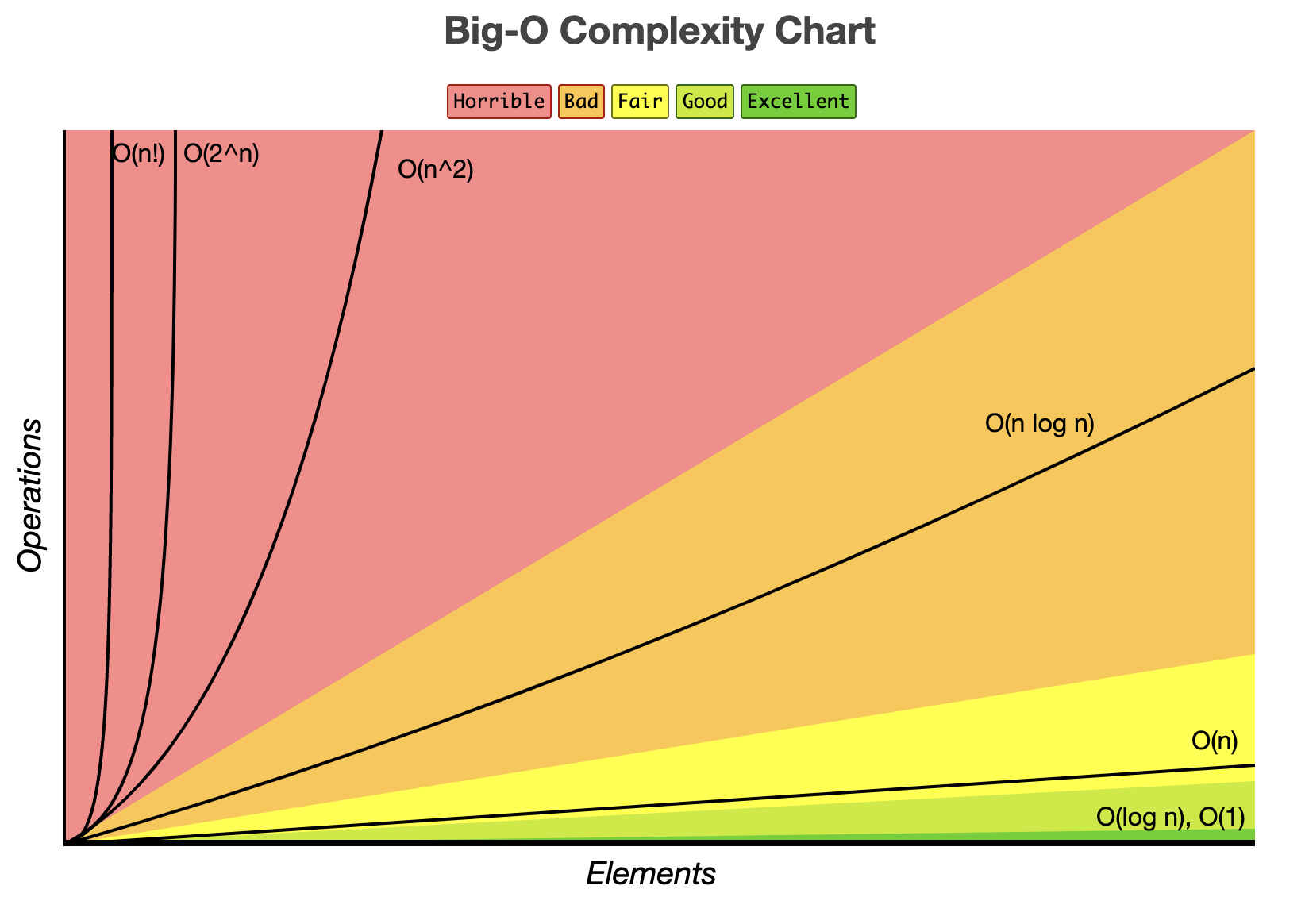 BigO Complexity Chart by https://www.bigocheatsheet.com
However I want to share with you my simple cheatsheet about big O notations. These just takes into account the most common ones, so if you need something deeper, please refer to links shared above
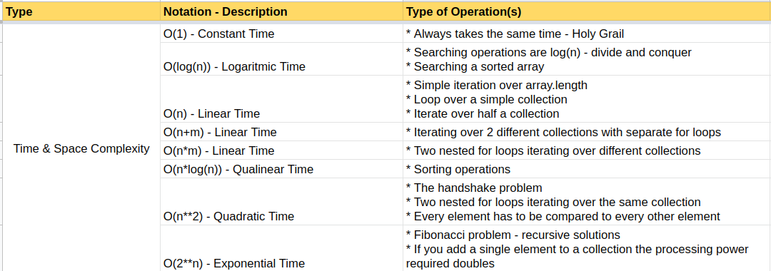
Worst Case Scenarios
Big O notation is usually understood to describe the worst-case scenario complexity algorithm, even though the worst-case complexity might differ from the average-case complexity. For example, some sporting algorithms have different time complexities depending on the layout of elements in their input array. Thus, when describing the time complexity of an algorithm, it can sometimes be helpful to specify whether the time complexity refers to the average case or the worst case
On our next blog post we’ll see the algorithms that operates in a logarithmic time and space, because they have something special and we need to learn about it
I hope you learned a lot with this post
Thanks for reading
DanielM